Turn away from the Sun.
Your shadow points toward the antisolar point, exactly opposite the Sun. With the Sun 15° above a level horizon, that point is 15° below it. Rain must lie along the useful sightlines; a dark cloud alone cannot make a rainbow.
An illustrated descent into optics
Follow the light. Change your point of view.
Keep going until rays become waves.
See / the everyday picture
A rainbow is sunlight redirected by many droplets into particular viewing directions; its position depends on the observer.
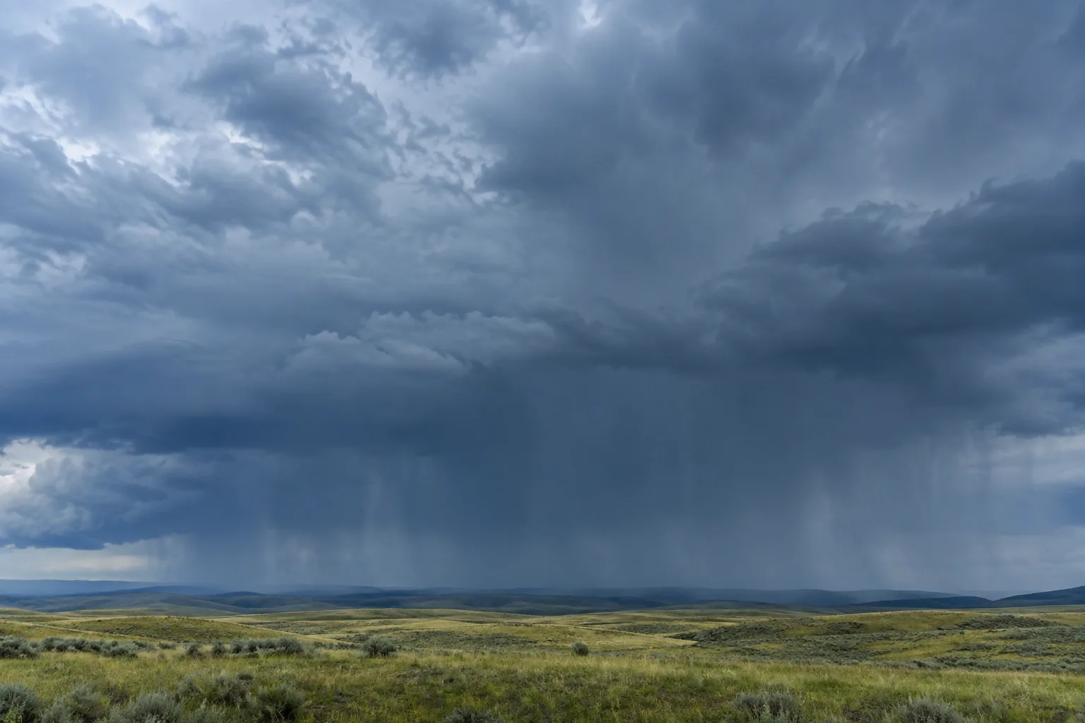
The Sun is behind your shoulder. Rain hangs ahead. A small fraction of the light entering those drops returns toward your eye. You see the directions where that light is concentrated.
Your shadow points toward the antisolar point, exactly opposite the Sun. With the Sun 15° above a level horizon, that point is 15° below it. Rain must lie along the useful sightlines; a dark cloud alone cannot make a rainbow.
Our ray presets sample 450, 550 and 650 nm, three points in a continuous spectrum. Water bends them by different amounts. The familiar color names are useful labels, not seven discrete components that arrive separately from the Sun.
A drop 100 m away and another 500 m away can lie along the same 42° sight direction. Those illustrative distances change no angle. The bow is not a colored object suspended at one fixed distance, so walking toward its end selects new light paths.
A constant angle around the antisolar axis makes a circle of directions. At a level ground horizon, a 15° Sun leaves the top of a roughly 42° bow about 27° high. From above droplets, more of the circle can be visible; altitude alone does not supply missing rain.
Look back at the opening: the Sun belongs behind the viewpoint. The bow’s center belongs in the opposite direction. Geometry source and derivation.
Trace / one small optical instrument
Follow one ray through a spherical water drop. The surface bends the transmitted light twice and partially reflects it once.
1Refraction on entryLight entering water bends toward the surface normal.
2Partial internal reflectionA fraction returns into the drop. Other light transmits out.
3Refraction on exitLight leaving water bends away from the normal, toward a possible observer.
Incidence i and refraction r are measured from the surface normal, not the tangent. In the ideal n = 4/3 rainbow ray, i = 59.391° becomes r = 40.203°. A ray aimed through the center has zero incidence and no entry bending.
At 20°C and density 998.2 kg/m³, the IAPWS relation gives about 1.33961 at 450 nm and 1.33167 at 650 nm. Here the surrounding index is idealized as 1. These values are not a color-to-screen conversion; the line colors identify wavelengths. [Water data]
For n = 4/3, the water-to-air critical angle is 48.590°. The primary ray reaches the reflecting surface at 40.203°, below that threshold. Partial reflection is enough. Drawing all the incident energy bouncing would give the wrong brightness story.
The ideal ray turns through 137.970° between its incoming and outgoing propagation vectors. Its apparent radius is the supplementary 42.030°. One drop scatters into many directions; one eye in one place does not receive that drop’s entire visible rainbow.
Checkpoint: name the three events before continuing: entry refraction → partial reflection → exit refraction.
Locate / the observer matters
Keep the rain field fixed. Move your eye. The directions that connect droplets to you change.
650 nm ray geometry. Sampling highlights fixed drops in the 1° band immediately inside the cone edge; that band is an illustration aid, not a physical cutoff. Distances are normalized, and the wireframe below the ground is a geometric extension. Link to this plate · Download the vector plate.
The antisolar direction is 180° from the Sun. Raise the Sun from 15° to 30° and the axis tilts down by another 15°. It is a direction in your own sky, not a particular droplet; angular observations use the same frame discipline as celestial navigation.
Rotating a sightline through every azimuth at radius β gives a cone with your eye at its apex. A cross-section at any distance is circular; the drop distances need not match. The 42° label refers to the cone’s half-angle, not an 84° angle from its axis.
For a level ground horizon, the top is approximately β minus Sun elevation. At 45° elevation, the primary construction lies below that horizon. An elevated observer looking down into spray or rain can still see a bow below eye level, potentially a full circle if droplets fill all the directions.
A and B are separated by 1.2 illustrative units. Their red-light cones select different samples in the same rain field. Some contributing regions may overlap, especially with finite wavelength and angular ranges; “no two people ever receive light from a common drop” is too strong.
Sunlight enters droplets, partly reflects, and exits. Dispersion separates the preferred directions by wavelength. Your eye selects a circular family of directions, and the horizon usually hides part of it.
Keep going: why does the concentration occur near 42°? →Derive / the optical bench
Change where a ray hits the drop. Most outgoing directions change quickly. Near one particular impact parameter, neighboring rays leave in almost the same direction.
With external index 1, the sine of incidence equals n times the sine of refraction. Angles are to the normal. The controls use temperature-specific dispersion; the worked derivation below deliberately uses constant n = 4/3.
a is drop radius and b is the incoming ray’s offset from its center. At u = 0.5, i = 30°. Restricting the control to 0–0.99 avoids the exactly tangent boundary; offset is a length ratio, not an angle.
For the primary, the accumulated turn lies between 0 and π and is also the scattering angle θ. Its minimum is about 138°. The apparent rainbow radius β = π − θ is therefore a maximum near 42°. This conversion changes for higher orders. [Ray conventions]
At the stationary ray, the first derivative dθ/di is zero. A small input change then changes θ only at second order. The ray-density model predicts a caustic, with formally divergent intensity. That identifies concentration, not an infinitely bright physical sky.
Differentiate the deflection and use Snell’s law: at the stationary point, n cos r = 2 cos i.
Then u = √(20/27) = 0.860663, i = 59.391102°, and r = 40.202966°.
θ = 137.970341° → β = 42.029659°
Calculated values for an ideal constant index, not six-decimal predictions of a real atmosphere. Reproduce with node scripts/rainbow/check.cjs.
Checkpoint: select b/a = 0.5. Its exit ray still exists, but it is not the rainbow’s stationary ray.
Compare / another path through the same drop
The secondary bow belongs to rays that reflect twice inside a drop. The extra event changes both the angle and the wavelength ordering.
Each internal reflection returns only part of the incident energy. A two-reflection path is therefore usually weaker than the primary under comparable conditions. Visibility also depends on the background and illumination, so counting reflections alone does not predict a photograph’s brightness.
With one reflection, stronger blue bending leads to a smaller primary radius. With two, it leads to a larger secondary radius. Red lies outside the primary and inside the secondary. The diagram’s labeled paths matter more than any particular display’s color rendition.
The secondary’s ideal accumulated deflection is 230.978°. Its physical scattering angle is arccos(cos Θ) = 129.022°, giving β = 50.978°. Directly subtracting 230.978° from 180° would incorrectly produce a negative radius.
The primary ray family concentrates light inside its outer boundary; the secondary family contributes outside its inner boundary. Between roughly 42° and 51°, those dominant ray families leave a deficit. Diffuse sky light, other scattering paths and wave tails keep the gap from being black.
| Phenomenon | Optical mechanism | Region & color behavior | Diagnostic feature | Limitation |
|---|---|---|---|---|
| Primary | Refraction → one internal reflection → refraction. | Near 42° from antisolar; red outside violet. | Usually stronger than the secondary in comparable conditions. | Angle alone predicts neither brightness nor fringes. |
| Secondary | Two internal reflections between entry and exit. | Roughly 51°; red inside violet. | Reversed colors and a darker gap toward the primary. | Angle depends on wavelength and index; extra reflections do not guarantee visibility. |
| Supernumerary | Wave interference near a rainbow caustic. | Additional bands inside the primary; spacing depends on size. | Fine repeated fringes, not a separate reflection order. | Size and source averaging can erase them. |
| Fogbow | Broad wave scattering pattern from small droplets. | A broad pale bow near the primary region. | Weak color separation compared with its width. | No single size threshold predicts appearance for all distributions. |
| Higher orders | Three or more internal reflections. | The tertiary can occur around 40° from the Sun, on the sunward side. | Location differs from the familiar antisolar pair. | Glare, background and droplet shape strongly affect visibility. [Higher orders] |
| Glory | Wave backscattering by droplets; multiple contributions. | Small colored rings near the antisolar point. | Often surrounds the observer’s shadow on a cloud. | It is not the 42° primary compressed into a smaller circle. [Glory] |
Resolve / rays become waves
Ray geometry locates a concentration. Wave optics makes its intensity finite and introduces fringes. These are calculations at one wavelength, not a full-color rainbow simulation.
Choose a calculated radius. The angular scale grows as radius decreases. The fine ripples of complete sphere scattering also include interference between paths omitted by the single-family Airy approximation.
Original Airy theory is a qualitative approximation for these presets. Independent peak normalization is not an accuracy fit. [Approximation limits]
Near the stationary point, θ − θR is proportional to (u − uR)². Inverting that map gives a ray-density factor proportional to 1/√(θ − θR) on the lit side. Its infinite edge is a model singularity, not a physical energy source.
The scaled coordinate is z = (β − βR)/δ, with both angular quantities in radians and δ = h1/3/x2/3. Here x = 2πa/λ, where a is drop radius and λ the exterior wavelength. The factor h is half the local deflection curvature, 4.927462 for n = 1.332; its derivation follows below. At the geometric edge z = 0, Ai(0)² = 0.126045. Finite intensity replaces the divergence; this normalized function alone has no absolute brightness units.
For the 100 μm, 650 nm, n = 1.332 case, δ = 0.997285°. The first Airy maximum at z = −1.018793 falls at β = 41.2077°, inside the geometric 42.2238° edge. At 25 μm, δ grows to 2.5130°. A broad size distribution averages different fringe spacings together.
Perpendicular means the electric field is normal to the plane containing incident and scattered directions; parallel means it lies in that plane. The two Mie amplitudes give different patterns. Near some minima the usual dominance can reverse, so one polarization curve is not a universal substitute for both.
Checkpoint: ordinary ray tracing cannot predict the extra interference bands. Their absence outdoors need not mean the wave calculation is wrong; the illumination and drop population may average them out.
Calculate / make the assumptions executable
Start with an isolated homogeneous sphere and a monochromatic plane wave. Then decide which features of an actual sky must be averaged over.
a is radius and λ is wavelength in the surrounding medium. At a = 100 μm and λ = 0.650 μm, x = 966.643893. The wave examples use real relative index 1.332 to reproduce a published case, not the separate IAPWS ray preset. Zero imaginary index excludes absorption.
Lorenz–Mie theory matches electromagnetic boundary conditions at the sphere. For our convention, |S₁(θ)|² and |S₂(θ)|² are the perpendicular and parallel angular intensities; their mean is the unpolarized intensity. At physical distance R, the irradiance factor includes 1/(kR)², k = 2π/λ. The plot is not irradiance at your eye.
The Debye decomposition reorganizes scattering contributions: p = 0 contains external reflection and diffraction, p = 1 direct transmission, p = 2 one internal reflection, p = 3 two. It is a decomposition of the sphere solution, not a competing physical theory. Our plotted Mie curve sums all contributions; it is not an isolated p = 2 curve.
A single-drop plane-wave calculation needs additional intensity averages over drop sizes, the finite solar disk (about 0.5° across), and wavelength before resembling daylight. Fine structure can disappear at each stage. A color rendering additionally needs an illuminant, color-matching functions and gamut rules; these plots deliberately remain monochromatic. [Reference case]
Inputs: radius 100 μm, wavelength 650 nm, relative index 1.332 + 0i, exterior index 1, scattering angle 140° (β = 40°), monochromatic plane wave. No size, source-disk or spectral averaging.
|S₁|² = 32093.46950
|S₂|² = 85537.50750
These are dimensionless amplitude-squared values in the Wiscombe convention: the unpolarized angular integral is πx²Qsca. The parallel value exceeds the perpendicular value at this particular angle; do not infer a whole-bow brightness ratio from one sample.
Compute: python scripts/rainbow/compute.py. The committed sample grid is β = 35–43° in 0.01° steps. The 100 μm inputs match Laven’s Fig. 2(a); its plotted curve is perpendicular. Validation uses a published MIEV0 benchmark plus independent direct Riccati–Bessel sums, not visual tracing of the paper. Reproduction and error record.
For S₂, swap πℓ and τℓ inside each term. The coefficients aℓ, bℓ enforce the sphere boundary conditions using spherical Bessel functions; they are not the radius a or impact parameter b. πℓ and τℓ are angular functions of cos θ. The development script spells out their recurrence and an independent coefficient evaluation. Complex amplitudes depend on time-sign convention; the reported squared magnitudes do not.
| Model | Inputs | Predicts | Cannot predict | Use when |
|---|---|---|---|---|
| Geometric rays | Sphere, index, incidence; n = 4/3 in our ideal example. | Paths and stationary deflection. | Interference or finite caustic intensity. | Locating the ray concentration; switch for fringes. |
| Airy approximation | Size, index, local deflection curvature and amplitude assumptions. | Finite fold profile and fringe scale. | All ray families or exact small-drop intensities. | Understanding near-caustic wave structure; check its validity range. |
| Lorenz–Mie | Homogeneous sphere, complex relative index, x, plane-wave illumination. | Full vector scattering for that sphere. | Arbitrary shapes, multiple scattering or an unmodeled atmosphere. | Requiring the full single-sphere angular pattern. |
| Debye decomposition | The sphere problem, with contributions indexed by internal reflections. | Separation and interference of selected path families. | A new nonspherical theory or automatic daylight averaging. | Comparing a primary approximation with the corresponding p = 2 contribution. |
| Nonspherical numerical scattering | Shape, orientation, size, material, illumination, converged discretization. | Shape-dependent patterns under the chosen solver assumptions. | Accuracy without convergence checks; all scales at equal cost. | Testing oblate or irregular drops with a suitable wave solver or validated wavefront method. |
Investigate / the research notebook
The sphere is exceptionally useful. It is still a sphere. Changing the question can require changing the method, not merely adjusting a slider.
A sphere has aspect ratio 1. An oblate test shape with vertical/horizontal ratio 0.95 breaks that symmetry and may shift or split angular features. That is an investigation input, not a measured rain population. The spherical Mie curves above cannot compute this change. [Shape methods]
For the tertiary, p = 4 means three internal reflections. Its familiar predicted location is sunward, around 40° from the Sun rather than from the antisolar point. Background contrast and drop shape affect visibility. Higher order does not mean simply “another concentric band outside the secondary.” [Visibility study]
A fold caustic is where two stationary-phase contributions coalesce. Keeping the local cubic phase instead of treating the two rays separately produces an Airy function. This step needs large x, a smooth amplitude, a small angular neighborhood and an isolated fold; it is not a global replacement for Maxwell’s equations.
Our sphere check adds 20 multipole orders and compares every sampled angle. The largest peak-relative intensity change is below 4.9 × 10⁻⁸. This tests series truncation for three specified cases. It does not establish angular-grid convergence for every possible drop or validate an uncomputed nonspherical case.
E is field amplitude, A is a slowly varying amplitude factor, x = 2πa/λ is size parameter, and Φ is dimensionless phase. Here u is the offset from the stationary normalized impact parameter, and Δ = θ − θR is in radians.
The stationary condition becomes h u² − Δ = 0. For Δ > 0, two real paths exist; at Δ = 0 they merge. Here h is half the second derivative of primary deflection with respect to normalized impact parameter at the stationary ray. For n = 1.332, h = 4.927462.
Replace A(u) by its local constant A(0). After dropping a common phase, the integral is proportional to ∫exp[i(t³/3 + zt)]dt = 2πAi(z). Thus E ≈ 2πA(0)Ai(z)/(xh)1/3, and intensity follows Ai(z)².
Higher phase terms, amplitude variation, other Debye families and nonspherical geometry were left out. The original Airy shape above is not the generalized Airy theory that also retains derivative terms. Compare like contributions and state the angular region before declaring agreement. [Derivation and validity]
Experiment A
Change: lognormal radius spread from 0% to 1% to 10%, median 100 μm, λ = 650 nm.
Predict: reduced fine-fringe contrast. Method: weighted Mie intensity averages, doubling size quadrature until stable.
Failure criterion: a claimed contrast trend changes when the quadrature doubles. This average has not been computed on this page.
Experiment B
Change: p = 2 to p = 3 at x = 500, 1000 and 5000.
Predict: different Airy approximation errors. Method: compare Airy with the same Debye contribution in a ±2° caustic window.
Failure criterion: peak-relative error exceeds a chosen 5% investigation target. Full Mie versus primary Airy is not this test.
Experiment C
Change: equal-volume sphere to vertical aspect ratios 0.98 and 0.95; equivalent radius 25 μm, λ = 650 nm.
Predict: azimuth-dependent shifts. Method: a converged nonspherical solver, such as an applicable T-matrix implementation.
Failure criterion: the shift is no larger than the estimated numerical error. These outcomes are uncomputed, not hidden Mie presets.
Check your picture
A bow is an angular pattern centered on your viewing geometry. It has no one distance to reach.
Different viewing directions select different drops. A drop sends different parts of its scattered pattern elsewhere.
The primary requires two refractions and one internal reflection. Refraction alone is a different path.
The ideal primary’s 40.203° internal incidence is below its 48.590° critical angle.
The spectrum is continuous. Color names and our six design accents are not physical partitions.
Measure the primary radius from the antisolar direction. The corresponding scattering angle is about 138°.
Alexander’s band is a relative deficit. Other scattering and background light remain.
The sphere solution assumes a sphere. An oblate drop changes the boundary-value problem.
Continue the investigation
Source links checked during production on September 19, 2026. Calculated diagrams are original; cited figures supplied parameters and conventions, not copied artwork.
